Note:
You can download this demo as a Jupyter notebook here and run it interactively yourself. The PolyChord nested sampling run data it uses can be downloaded at https://github.com/ejhigson/nestcheck_demo_data (this also contains runs using a few other likelihoods).
Quickstart demo
This is a brief demonstration covering loading nested sampling run data, performing calculations, running error analysis and diagnostic tests, and making plots. For detailed explanations of the diagnostic tests and plots, see the papers which introduce them (Higson et al. 2018, Higson et al. 2019).
More information about nestcheck’s code and and functionality can be found in the documentation. For more examples of nestcheck’s usage, including on a variety of likelihoods, see code used to make the results and diagrams in the diagnostic tests paper (Higson et al. 2019) (available at https://github.com/ejhigson/diagnostic).
Loading nested sampling runs
For this demo we will use some PolyChord nested sampling runs with a simple 2-dimensional Gaussian likelihood
with \(\sigma=0.5\) and a uniform prior on each parameter in \([-10, 10]\). For more information about the dictionary format and keys nestcheck uses to store nested sampling runs, see the API documentation.
For example, a PolyChord run can be loaded as follows:
[1]:
import nestcheck.data_processing

base_dir = 'polychord_chains'  # directory containing run (PolyChord's 'base_dir' setting)
file_root = 'gaussian_2d_100nlive_5nrepeats_1'  # output files' name root (PolyChord's 'file_root' setting)
run = nestcheck.data_processing.process_polychord_run(file_root, base_dir)
nestcheck.data_processing also has functions for loading nested sampling data from a variety of nested sampling software packages (including MultiNest), and you can add your own method to load data from other sources.
Data from multiple runs can be loaded and processed together (with optional parallelisation):
[2]:
file_roots = ['gaussian_2d_100nlive_5nrepeats_' + str(i) for i in range(1, 11)]
run_list = nestcheck.data_processing.batch_process_data(
    file_roots, base_dir=base_dir, parallel=True,
    process_func=nestcheck.data_processing.process_polychord_run)
Evidence and parameter estimation calculations from runs
Nested sampling runs in the nestcheck format can be easily used to make posterior inferences (see estimators.py for more example functions)
[3]:
import nestcheck.estimators as e

print('The log evidence estimate using the first run is',
      e.logz(run_list[0]))
print('The estimateed the mean of the first parameter is',
      e.param_mean(run_list[0], param_ind=0))
The log evidence estimate using the first run is -5.941675954408192
The estimateed the mean of the first parameter is 0.003249535192363336
You can get a pandas DataFrame of results for a list of quantities and a list of runs as follows:
[4]:
import nestcheck.diagnostics_tables

estimator_list = [e.logz, e.param_mean, e.param_squared_mean, e.r_mean]
# Use nestcheck's stored LaTeX format estimator names
estimator_names = [e.get_latex_name(est) for est in estimator_list]
vals_df = nestcheck.diagnostics_tables.estimator_values_df(
    run_list, estimator_list, estimator_names=estimator_names)
vals_df
[4]:
| $\mathrm{log} \mathcal{Z}$ | $\overline{\theta_{\hat{1}}}$ | $\overline{\theta^2_{\hat{1}}}$ | $\overline{|\theta|}$ | |
|---|---|---|---|---|
| run | ||||
| 0 | -5.934184 | -0.000376 | 0.242457 | 0.625360 |
| 1 | -5.941676 | 0.003250 | 0.238832 | 0.594131 |
| 2 | -5.997774 | -0.017127 | 0.263610 | 0.629681 |
| 3 | -5.848036 | -0.026617 | 0.279740 | 0.654915 |
| 4 | -5.761255 | -0.004223 | 0.230528 | 0.608089 |
| 5 | -5.874927 | -0.012669 | 0.224504 | 0.598055 |
| 6 | -5.784370 | 0.011934 | 0.249281 | 0.599508 |
| 7 | -5.880606 | 0.019924 | 0.253596 | 0.616933 |
| 8 | -6.297974 | 0.031247 | 0.264749 | 0.663862 |
| 9 | -5.863086 | -0.031087 | 0.257504 | 0.648641 |
Bootstrap sampling error estimates
The sampling error on calculations from nested sampling runs can be estimated using the bootstrap approach method introduced in Higson et al. (2018) Section 4 (see the paper for more details).
[5]:
import pandas as pd
import nestcheck.error_analysis

bs_error_df = pd.DataFrame(columns=estimator_names)
for i, run in enumerate(run_list[:2]):  # just use the first two runs as an example
    bs_error_df.loc[i] = nestcheck.error_analysis.run_std_bootstrap(run, estimator_list, n_simulate=100)
bs_error_df.index.name = 'run'
print('Run boostrap error estimates:')
bs_error_df
Run boostrap error estimates:
[5]:
| $\mathrm{log} \mathcal{Z}$ | $\overline{\theta_{\hat{1}}}$ | $\overline{\theta^2_{\hat{1}}}$ | $\overline{|\theta|}$ | |
|---|---|---|---|---|
| run | ||||
| 0 | 0.193681 | 0.026585 | 0.016430 | 0.022041 |
| 1 | 0.214706 | 0.025536 | 0.019318 | 0.020765 |
Diagrams of uncertainties on posterior distributions using bootstrap resamples
Bootstrap resamples of nested sampling runs can be used to plot numerical uncertainties on whole posterior distributions (rather than just scalar quantities) using nestcheck’s bs_param_dists function.
[6]:
import nestcheck.plots
%matplotlib inline

fig = nestcheck.plots.bs_param_dists(run_list[:2])
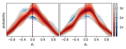
Here the dashed dark red and dark blue lines mark the estimates of the mean of each parameter for the red and blue runs respectively. For a detailed explanation of this type of diagram and its uses, see Higson et al. (2019) Section 4.1 and Figure 3.
Diagrams of samples in log X
The param_logx_diagram function plots nested sampling diagrams of the type proposed in Higson et al. (2019) Section 4.2 and shown in Figures 4 and 5.
[7]:
fig = nestcheck.plots.param_logx_diagram(run_list[0], logx_min=-15)
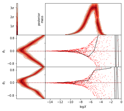
These diagrams illustrate the nested sampling algorithm’s exponential compression of the prior by plotting samples in \(\log X\), where \(X(\mathcal{L}) \in [0, 1]\) is the fraction of the prior with likelihood greater than \(\mathcal{L}\). The algorithm iterates towards higher likelihoods (towards lower \(\log X\) values). The plots on the left are similar the distributions plotted in the previous cell, and the top right plot shows the relative posterior mass at each \(\log X\) value. See Higson et al. (2019) Section 4.2 for a detailed explanation and more examples.
Calculating errors due to implementation-specific effects
Nested sampling software used for practical problems, such as MultiNest and PolyChord, uses numerical techniques to produce approximately uncorrelated samples within some iso-likelihood contour. However, for challenging problems - such as those with multimodal or degenerate posteriors - the software may fail to do this accurately, causing additional errors due to implementation-specific effects (see Higson et al. 2019 for more details).
The error due to implementation-specific effects can be estimated with nestcheck using the method described in Section 5 of Higson et al. (2019). This involves computing the standard deviation of results from repeated calculations, and therefore requires multiple runs (the more runs used, the more precise the results).
[8]:
df = nestcheck.diagnostics_tables.run_list_error_summary(run_list, estimator_list, estimator_names, 100)
df
[8]:
| $\mathrm{log} \mathcal{Z}$ | $\overline{\theta_{\hat{1}}}$ | $\overline{\theta^2_{\hat{1}}}$ | $\overline{|\theta|}$ | ||
|---|---|---|---|---|---|
| calculation type | result type | ||||
| values mean | value | -5.918389 | -0.002574 | 0.250480 | 0.623917 |
| uncertainty | 0.047744 | 0.006330 | 0.005339 | 0.007926 | |
| values std | value | 0.150980 | 0.020019 | 0.016884 | 0.025065 |
| uncertainty | 0.035586 | 0.004718 | 0.003980 | 0.005908 | |
| bootstrap std mean | value | 0.217638 | 0.026168 | 0.018131 | 0.022129 |
| uncertainty | 0.010354 | 0.000704 | 0.000481 | 0.000441 | |
| implementation std | value | 0.000000 | 0.000000 | 0.000000 | 0.011771 |
| uncertainty | 0.055952 | 0.009373 | 0.010334 | 0.014222 | |
| implementation std frac | value | 0.000000 | 0.000000 | 0.000000 | 0.469616 |
| uncertainty | 6.940037 | 2.363760 | 1.141478 | 1.763814 |
The 2-dimensional Gaussian likelihood is unimodal and easy for PolyChord to sample, so as expected we see that the standard deviation of the result values is close to the mean bootstrap standard deviation. Consequently the estimated errors due to implementation-specific effects are low.
Tests for implementation specific effects using only 2 nested sampling runs
It is impossible to tell a priori if implementation-specific effects are present in a single nested sampling run without some additional knowledge of what the results should be. However diagnostic tests to determine if significant implementation-specific effects are present using only two nested sampling runs are proposed in Higson et al. (2019).
The first test divides nested sampling runs into their constituent single live point runs (“threads”) and assesses whether threads within each run are correlated with each other using the Kolmogorov–Smirnov test. This yields a \(p\)-value, with \(p \approx 0\) indicating implementation-specific effects are almost certainly present.
Secondly, the statistical distance between the uncertainty distributions (calculated from bootstrap replications) of quantities such as \(\log X\) or parameter means for the two runs can be calculated. We use the Kolmogorov–Smirnov statistic as a distance measure; if this is close to 1 then there little or is no overlap between the distributions and additional errors from implementation-specific effects are likely present.
For a full explanation see the diagnostic tests paper (Higson et al. 2019)).
These statistcs can be computed for pairs of runs using nestcheck as:
[9]:
# perform error analysis on two runs
error_vals_df = nestcheck.diagnostics_tables.run_list_error_values(
    run_list[:2], estimator_list, estimator_names, thread_pvalue=True, bs_stat_dist=True, n_simulate=100)
# select only rows containing pairwise tests to output
error_vals_df.loc[pd.IndexSlice[['thread ks pvalue', 'bootstrap ks distance'], :], :]
[9]:
| $\mathrm{log} \mathcal{Z}$ | $\overline{\theta_{\hat{1}}}$ | $\overline{\theta^2_{\hat{1}}}$ | $\overline{|\theta|}$ | ||
|---|---|---|---|---|---|
| calculation type | run | ||||
| thread ks pvalue | (1, 0) | 0.343886 | 0.556017 | 0.67662 | 0.260553 |
| bootstrap ks distance | (1, 0) | 0.190000 | 0.290000 | 0.58000 | 0.570000 |
As expected, the \(p\)-values are not particularly low nor are the KS distances particularly high - indicating there are no significant implementation-specific effects for the simple 2-dimensional Gaussian.
If more than two runs are provided, the above function will calculate the diagnostics for each pairwise combination.